Parametric Bootstrap on Distributions Fitted with Maximum Likelihood

The parametric bootstrap is a resampling technique using random variates from a known parametric distribution. In this function the distribution of the random variates is completely determined by the unvariateML object object.

Usage

bootstrapml(
  object,
  reps = 1000,
  map = identity,
  reducer = stats::quantile,
  ...
)

Arguments

object: A univariateML object.
reps: Positive integer. The number of bootstrap samples.
map: A function of the parameters of the univariateML object. Defaults to the identity.
reducer: A reducer function. Defaults to stats::quantile with default argument probs = c(0.025, 0.975).
...: Passed to reducer.

Value

The transposed map-reduced bootstrap samples.

Details

For each bootstrap iteration a maximum likelihood estimate is calculated using the ml*** function specified by object. The resulting numeric vector is then passed to map. The values returned by map is collected in an array and the reducer is called on each row of the array.

By default the map function is the identity and the default reducer is the quantile function taking the argument probs, which defaults to c(0.025, 0.975). This corresponds to a 95\ basic percentile confidence interval and is also reported by confint()

Note: The default confidence intervals are percentile intervals, not empirical intervals. These confidence intervals will in some cases have poor coverage as they are not studentized, see e.g. Carpenter, J., & Bithell, J. (2000).

References

Efron, B., & Tibshirani, R. J. (1994). An introduction to the bootstrap. CRC press.

Carpenter, J., & Bithell, J. (2000). Bootstrap confidence intervals: when, which, what? A practical guide for medical statisticians. Statistics in medicine, 19(9), 1141-1164.

Examples

# \donttest{
set.seed(1)
object <- mlgamma(mtcars$qsec)

## Calculate c(0.025, 0.975) confidence interval for the gamma parameters.
bootstrapml(object)
#>            2.5%     97.5%
#> shape 70.285697 180.72290
#> rate   3.965363  10.12785

#            2.5%      97.5%
# shape 68.624945 160.841557
# rate   3.896915   9.089194

## The mean of a gamma distribution is shape/rate. Now we calculate a
## parametric bootstrap confidence interval for the mean with confidence
## limits c(0.05, 0.95)

bootstrapml(object, map = \(x) x[1] / x[2], probs = c(0.05, 0.95))
#>       5%      95% 
#> 17.33962 18.31253 

#       5%      95%
# 17.33962 18.31253

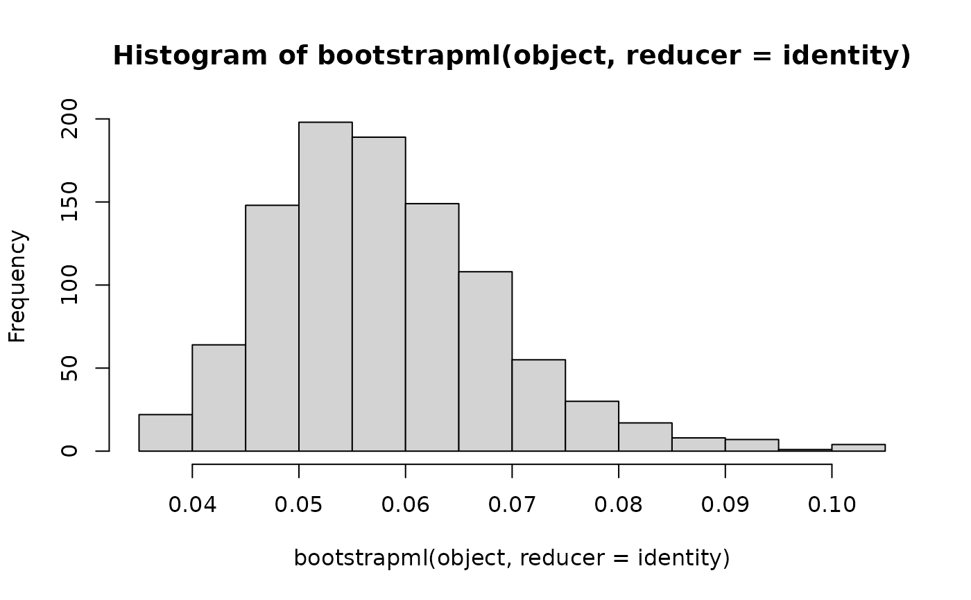
## Print a histogram of the bootstrapped estimates from an exponential.
object <- mlexp(mtcars$qsec)
hist(bootstrapml(object, reducer = identity))

# }