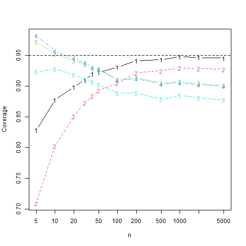
Simulation of confidence intervals.

Setting up the simulations

We use the dataset bfi from the package psych together with lavaan to estimate some realistic factor loadings $\lambda$ and standard deviations $\sigma$.

model <- c("y =~ A1 + A2 + A3 + A4 + A5")
fit <- lavaan::cfa(model, data = psych::bfi)
coefs <- lavaan::lavInspect(fit, what = "x")
lambda <- abs(c(coefs$lambda * sqrt(as.numeric(coefs$psi))))
sigma <- sqrt(diag(lavaan::lavInspect(fit, what = "x")$theta))

We take the absolute value of the lambda vector as the agreement data contains reverse-coded items.

Comparing confidence intervals coverages and lengths

We compare five confidence intervals, all without transformations. The adf interval is the asymptotic distribution-free interval, the ell interval is the interval based on elliptical distributions and a kurtosis correction, the ell_par is the elliptical interval assuming a parallel model. The same comments hold for norm (assuming normal data) and norm_par (assuming parallel normal data).

library("alphaci")
library("future.apply")
plan(multisession, workers = availableCores() - 2)
set.seed(313)

n_reps <- 10000
k <- 5
latent <- \(n) extraDistr::rlaplace(n) / sqrt(2)
true <- alphaci:::alpha(sigma, lambda)

In this simulation we normal error terms and a Laplace-distributed latent variable. This one has excess kurtosis $3$, which caries over in large part to the data. k is the number of questions ands n_reps is the number of simulations.

success <- \(ci) true <= ci[2] & true >= ci[1]
len <- \(ci) ci[2] - ci[1]
simulations <- \(n) {
    results  <- future.apply::future_replicate(n_reps, {
      x <- alphaci:::simulate_congeneric(n, k, sigma, lambda, latent = latent)
      cis <- rbind(adf = alphaci(x, type = "adf"),
        adf_par = alphaci(x, type = "adf", parallel = TRUE),
        ell = alphaci(x, type = "elliptical"),
        ell_par = alphaci(x, type = "elliptical", parallel = TRUE),
        norm = alphaci(x, type = "normal"),
        norm_par = alphaci(x, type = "normal", parallel = TRUE)
      )
      c(cov = apply(cis, 1, success), len = apply(cis, 1, len))
      }, future.seed = TRUE)
  rowMeans(results)
}

Let’s check out the results when $n= 10$.

simulations(10)
#>      cov.adf  cov.adf_par      cov.ell  cov.ell_par     cov.norm cov.norm_par      len.adf  len.adf_par 
#>    0.8745000    0.7942000    0.9513000    0.9566000    0.9223000    0.9297000    0.7680810   55.3239940 
#>      len.ell  len.ell_par     len.norm len.norm_par 
#>    1.0238478    1.0499270    0.9113473    0.9342908

It appears that the kurtosis corrections work well, at least for small sample size. Let’s see how they perform when $n$ increases.

nn <- c(5, 10, 20, 30, 40, 50, 100, 200, 500, 1000, 2000, 5000)
results <- sapply(nn, simulations)

Plotting the coverages, we find, where 1 is asymptotically distribution-free, 2 is elliptical, 3 is paralell and elliptical, 4 is normal and 5 is parallel and normal.

matplot(nn, t(results[1:5, ]), xlab = "n", ylab = "Coverage", type = "b",
        log = "x")
abline(h = 0.95, lty = 2)

Hence the kurtosis correction intervals have better coverage than the adf interval when $n\leq 50$ and outperforms the normal theory intervals for all $n$. If this observation is general remains to be seen.