Consistency with missing ratings

2023-05-02

The functions in quadagree are consistent in the presence of missing ratings, assuming every rater is the same, and the missingness does not depend on the data.

The following samples ratings from a Perreault-Leigh model where each rater has his own independent probability having his data missing. The inferential methods in quadagree are valid in more general settings that this, i.e., missingness might be depenent, or generated according to a suitable process (we only require that the process is mean-ergodic). The function simulate_jsm can be found at the bottom of this document.

#' Sample n rating vectors with missing data
#' @param n Number of vectors sampled.
#' @param p Probability vector with p[i] the probability that the ith raters
#'    data is not missing
sim <- \(n, p) {
  t_dist <- rep(1 / 5, 5)
  skills <- c(0.9, 0.1, 0.2, 0.5, 0.8, 0.9)
  x <- simulate_jsm(n, skills, model = "fleiss", true_dist = t_dist)
  for (i in seq_along(p)) x[sample(n, n - p[i] * n), i] <- NA
  x
}

Here is an example:

set.seed(313)
p <- c(0.9, 0.8, 0.7, 0.6, 0.5, 0.9)
x <- sim(10, p)
x

##       [,1] [,2] [,3] [,4] [,5] [,6]
##  [1,]    4    4    2    2   NA    4
##  [2,]    2   NA   NA   NA    5    2
##  [3,]    5    5    2   NA    1    5
##  [4,]    3    5    5    3   NA    3
##  [5,]   NA    5    3    5    4    4
##  [6,]    5    3    1    4   NA    5
##  [7,]    2    4    4    2    2    2
##  [8,]    4    3    2   NA   NA    4
##  [9,]    1   NA   NA    1    1    1
## [10,]    5    1   NA   NA   NA   NA
## attr(,"n")
## [1] 10
## attr(,"s")
## [1] 0.9 0.1 0.2 0.5 0.8 0.9
## attr(,"true_dist")
## [1] 0.2 0.2 0.2 0.2 0.2
## attr(,"guessing_dist")
## [1] 0.2 0.2 0.2 0.2 0.2
## attr(,"kappa")
## [1] 0.3

Observe the kappa attributes, which contains the true kappa (both Fleiss and Cohen). Now let’s estimate Fleiss using quadagree and irrCAC. The plot below shows the population value (solid line), the quadagree estimates (black), and the irrCAC estimates (blue).

set.seed(313)
kappa <- attr(x, "kappa")
n_reps <- 1000
nn <- c(50, 100, 250, 500, 750, 1000, 5000)
results <- sapply(nn, \(n) {
  results <- replicate(n_reps, {
    x <- sim(n, p)
    c(
      quadagree:::fleiss(x),
      c(irrCAC::fleiss.kappa.raw(x, weights = "quadratic")$est[4])$coeff.val
    )
  })
  rowMeans(results, na.rm = TRUE)
})

plot(nn, results[1, ],
  ylim = c(min(results, na.rm = TRUE), max(results, na.rm = TRUE)), type = "b",
  ylab = "Mean estimated kappa", xlab = "n"
)
points(nn, results[2, ], col = "blue", type = "b")
abline(h = kappa, lwd = 2)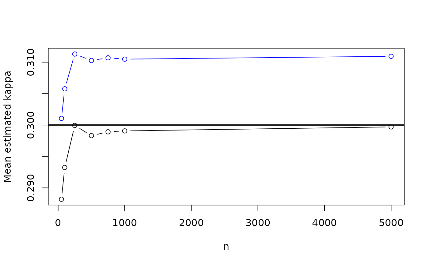

As can be seen, irrCAC has an asymptotic bias of approximately $0.11$, and is not consistent. quadagree approximates the true value better and better as $n$ grows larger.

Code for simulate_jsm

simulate_jsm <- \(n,
  s,
  model = c(
    "general",
    "cohen-fleiss",
    "fleiss",
    "bp",
    "tu"
  ),
  true_dist,
  guessing_dist) {
  model <- match.arg(model)

  if (model == "cohen-fleiss") {
    if (is.null(nrow(guessing_dist))) {
      true_dist <- guessing_dist
    } else {
      true_dist <- colSums(guessing_dist * (1 - s) / sum(1 - s))
    }
  } else if (model == "tu") {
    true_dist <- rep(1, ncol(guessing_dist)) / ncol(guessing_dist)
  } else if (model == "bp") {
    guessing_dist <- rep(1, length(true_dist)) / length(true_dist)
  } else if (model == "fleiss") {
    guessing_dist <- true_dist / sum(abs(true_dist))
  }

  if (any(true_dist < 0)) {
    stop("true_dist must contain only positive elements.")
  }

  # The true category for each item.
  q <- length(true_dist)
  x_star <- sample(q, n, replace = TRUE, prob = true_dist)

  if (is.null(nrow(guessing_dist))) {
    observations <- sapply(seq_along(s), function(j) {
      z <- stats::rbinom(n, 1, s[j])
      z * x_star + (1 - z) * sample(q, n, replace = TRUE, guessing_dist)
    })
  } else {
    observations <- sapply(seq_along(s), function(j) {
      z <- stats::rbinom(n, 1, s[j])
      z * x_star + (1 - z) * sample(q, n, replace = TRUE, guessing_dist[j, ])
    })
  }

  attr(observations, "n") <- n
  attr(observations, "s") <- s
  attr(observations, "true_dist") <- true_dist
  attr(observations, "guessing_dist") <- guessing_dist
  attr(observations, "kappa") <- true_jsm(s)
  observations
}

true_jsm <- \(s) {
  ss <- s %*% t(s)
  diag(ss) <- 0
  j <- ncol(ss)
  sum(ss) / (j * (j - 1))
}